Pandas 2: operazioni avanzate
Riferimenti: SoftPython - pandas 2
- visualizza al meglio in

- versione stampabile: clicca qua
- per navigare nelle slide: premere
Esc
Summer School Data Science 2023 - Modulo 1 informatica: Moodle
Docente: David Leoni david.leoni@unitn.it
Esercitatore: Luca Bosotti luca.bosotti@studenti.unitn.it
Raggruppare
Torniamo nello spazio con il dataset astropi.csv
Fonte: ESA / Raspberry foundation (abbiamo sostituito ROW_ID con time_stamp)
import pandas as pd
import numpy as np

df = pd.read_csv('astropi.csv', encoding='UTF-8')
- intervalli: interi, es da
42.0INCLUSO a43.0ESCLUSO
- come contare / fare statistiche in genere: con
groupby
- nota: per istogrammi in particolare ci sono modi più rapidi con numpy
Un gruppo d'esempio
Il 42 quante righe ha?
df[ df['humidity'].transform(int) == 42].head()
| time_stamp | temp_cpu | temp_h | temp_p | humidity | pressure | pitch | roll | yaw | mag_x | mag_y | mag_z | accel_x | accel_y | accel_z | gyro_x | gyro_y | gyro_z | reset | |
|---|---|---|---|---|---|---|---|---|---|---|---|---|---|---|---|---|---|---|---|
| 19222 | 2016-02-18 16:37:00 | 33.18 | 28.96 | 26.51 | 42.99 | 1006.10 | 1.19 | 53.23 | 313.69 | 9.081925 | -32.244905 | -35.135448 | -0.000581 | 0.018936 | 0.014607 | 0.000563 | 0.000346 | -0.000113 | 0 |
| 19619 | 2016-02-18 17:43:50 | 33.34 | 29.06 | 26.62 | 42.91 | 1006.30 | 1.50 | 52.54 | 194.49 | -53.197113 | -4.014863 | -20.257249 | -0.000439 | 0.018838 | 0.014526 | -0.000259 | 0.000323 | -0.000181 | 0 |
| 19621 | 2016-02-18 17:44:10 | 33.38 | 29.06 | 26.62 | 42.98 | 1006.28 | 1.01 | 52.89 | 195.39 | -52.911983 | -4.207085 | -20.754475 | -0.000579 | 0.018903 | 0.014580 | 0.000415 | -0.000232 | 0.000400 | 0 |
| 19655 | 2016-02-18 17:49:51 | 33.37 | 29.07 | 26.62 | 42.94 | 1006.28 | 0.93 | 53.21 | 203.76 | -43.124080 | -8.181511 | -29.151436 | -0.000432 | 0.018919 | 0.014608 | 0.000182 | 0.000341 | 0.000015 | 0 |
| 19672 | 2016-02-18 17:52:40 | 33.33 | 29.06 | 26.62 | 42.93 | 1006.24 | 1.34 | 52.71 | 206.97 | -36.893841 | -10.130503 | -31.484077 | -0.000551 | 0.018945 | 0.014794 | -0.000378 | -0.000013 | -0.000101 | 0 |
df[ df['humidity'].transform(int) == 42].shape
(2776, 19)
A ciascuno il suo gruppo
Creiamo una colonna che assegna a ciascuna riga il proprio gruppo:
df['humidity_int'] = df['humidity'].transform( lambda x: int(x) )
df[ ['time_stamp', 'humidity_int', 'humidity'] ].head()
| time_stamp | humidity_int | humidity | |
|---|---|---|---|
| 0 | 2016-02-16 10:44:40 | 44 | 44.94 |
| 1 | 2016-02-16 10:44:50 | 45 | 45.12 |
| 2 | 2016-02-16 10:45:00 | 45 | 45.12 |
| 3 | 2016-02-16 10:45:10 | 45 | 45.32 |
| 4 | 2016-02-16 10:45:20 | 45 | 45.18 |
groupby
Calcoliamo la statistica desiderata per ogni gruppo:
- prima la colonna su cui raggruppare
'humidity_int' - poi la colonna su cui effettuare la statistica
'humidity' - infine la statistica da calcolare, es
.count()- altre:
sum(),min(),max(), mediamean()...
- altre:
df.groupby(['humidity_int'])['humidity'].count()
humidity_int
42     2776
43     2479
44    13029
45    32730
46    35775
47    14176
48     7392
49      297
50      155
51      205
52      209
53      128
54      224
55      164
56      139
57      183
58      237
59      271
60      300
Name: humidity, dtype: int64
groupby - il risultato
risultato = df.groupby(['humidity_int'])['humidity'].count()
type(risultato)
pandas.core.series.Series
risultato.index
Int64Index([42, 43, 44, 45, 46, 47, 48, 49, 50, 51, 52, 53, 54, 55, 56, 57, 58,
            59, 60],
           dtype='int64', name='humidity_int')
groupby - plottiamo
%matplotlib inline
import matplotlib as mpl
import matplotlib.pyplot as plt

plt.bar(risultato.index,
        risultato)

plt.xlabel('gruppi umidità')
plt.ylabel('conteggio')
plt.title('Distribuzione umidità')

# mostra le etichette come interi
plt.xticks(risultato.index,
           risultato.index)
# rimuove le linette in fondo
plt.tick_params(bottom=False)

plt.show()
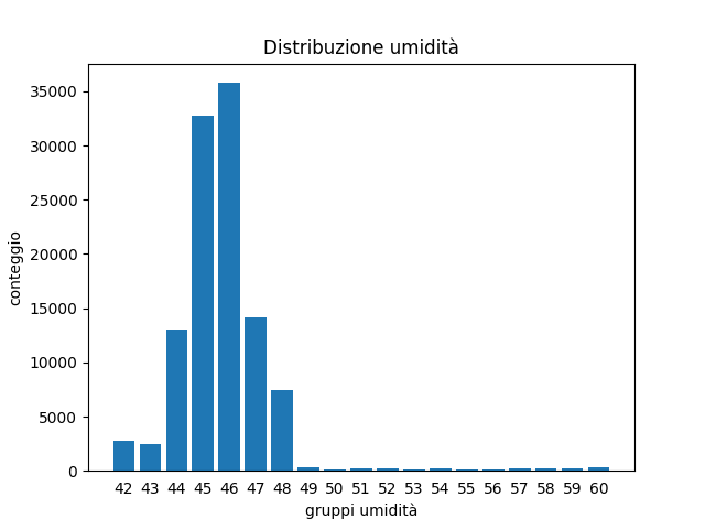
Problema: groupby produce poche righe
df.groupby(['humidity_int'])['humidity'].count()
humidity_int
42     2776
43     2479
44    13029
45    32730
46    35775
47    14176
48     7392
49      297
50      155
51      205
52      209
53      128
54      224
55      164
56      139
57      183
58      237
59      271
60      300
Name: humidity, dtype: int64
E se volessimo assegnare a ciascuna riga nella tabella originale il conteggio del proprio gruppo?
Per ogni riga, qual'è il conteggio del proprio gruppo?
df.groupby(['humidity_int'])['humidity'].transform('count')
0         13029
1         32730
2         32730
3         32730
4         32730
          ...
110864     2776
110865     2776
110866     2776
110867     2776
110868     2776
Name: humidity, Length: 110869, dtype: int64
Per ogni riga, salva il conteggio del proprio gruppo
nuova_colonna = df.groupby(['humidity_int'])['humidity'].transform('count')
df['Conteggio umidità'] = nuova_colonna
Verifichiamo:
df[['time_stamp', 'humidity_int', 'humidity', 'Conteggio umidità']]
| time_stamp | humidity_int | humidity | Conteggio umidità | |
|---|---|---|---|---|
| 0 | 2016-02-16 10:44:40 | 44 | 44.94 | 13029 |
| 1 | 2016-02-16 10:44:50 | 45 | 45.12 | 32730 |
| 2 | 2016-02-16 10:45:00 | 45 | 45.12 | 32730 |
| 3 | 2016-02-16 10:45:10 | 45 | 45.32 | 32730 |
| 4 | 2016-02-16 10:45:20 | 45 | 45.18 | 32730 |
| ... | ... | ... | ... | ... |
| 110864 | 2016-02-29 09:24:21 | 42 | 42.94 | 2776 |
| 110865 | 2016-02-29 09:24:30 | 42 | 42.72 | 2776 |
| 110866 | 2016-02-29 09:24:41 | 42 | 42.83 | 2776 |
| 110867 | 2016-02-29 09:24:50 | 42 | 42.81 | 2776 |
| 110868 | 2016-02-29 09:25:00 | 42 | 42.94 | 2776 |
110869 rows × 4 columns
Esercizi raggruppamento
Congiungere dataset
Date due tabelle che condividono una colonna, come congiungere le righe?
In pandas si può usare merge (o join)
Congiungere con merge: un esempio
il dataset iss-coords.csv contiene le coordinate della International Space Station (ISS):
iss_coords = pd.read_csv('iss-coords.csv', encoding='UTF-8')
iss_coords.head(3)
| timestamp | lat | lon | |
|---|---|---|---|
| 0 | 2016-01-01 05:11:30 | -45.103458 | 14.083858 |
| 1 | 2016-01-01 06:49:59 | -37.597242 | 28.931170 |
| 2 | 2016-01-01 11:52:30 | 17.126141 | 77.535602 |
Come mostrare le coordinate della ISS nel dataset originale astropi.csv?
df = pd.read_csv('astropi.csv', encoding='UTF-8')
df.head(3)
| time_stamp | temp_cpu | temp_h | temp_p | humidity | pressure | pitch | roll | yaw | mag_x | mag_y | mag_z | accel_x | accel_y | accel_z | gyro_x | gyro_y | gyro_z | reset | |
|---|---|---|---|---|---|---|---|---|---|---|---|---|---|---|---|---|---|---|---|
| 0 | 2016-02-16 10:44:40 | 31.88 | 27.57 | 25.01 | 44.94 | 1001.68 | 1.49 | 52.25 | 185.21 | -46.422753 | -8.132907 | -12.129346 | -0.000468 | 0.019439 | 0.014569 | 0.000942 | 0.000492 | -0.000750 | 20 |
| 1 | 2016-02-16 10:44:50 | 31.79 | 27.53 | 25.01 | 45.12 | 1001.72 | 1.03 | 53.73 | 186.72 | -48.778951 | -8.304243 | -12.943096 | -0.000614 | 0.019436 | 0.014577 | 0.000218 | -0.000005 | -0.000235 | 0 |
| 2 | 2016-02-16 10:45:00 | 31.66 | 27.53 | 25.01 | 45.12 | 1001.72 | 1.24 | 53.57 | 186.21 | -49.161878 | -8.470832 | -12.642772 | -0.000569 | 0.019359 | 0.014357 | 0.000395 | 0.000600 | -0.000003 | 0 |
Congiungere con merge: proviamo!
# ricorda che merge produce un NUOVO dataframe:

df = pd.read_csv('astropi.csv', encoding='UTF-8')

geo_astropi = df.merge(iss_coords, left_on='time_stamp', right_on='timestamp')

# merge aggiunge sia la colonna time_stamp che timestamp,
# perciò rimuoviamo la colonna duplicata 'timestamp'

geo_astropi = geo_astropi.drop('timestamp', axis=1)
geo_astropi
| time_stamp | temp_cpu | temp_h | temp_p | humidity | pressure | pitch | roll | yaw | mag_x | ... | mag_z | accel_x | accel_y | accel_z | gyro_x | gyro_y | gyro_z | reset | lat | lon | |
|---|---|---|---|---|---|---|---|---|---|---|---|---|---|---|---|---|---|---|---|---|---|
| 0 | 2016-02-19 03:49:00 | 32.53 | 28.37 | 25.89 | 45.31 | 1006.04 | 1.31 | 51.63 | 34.91 | 21.125001 | ... | -14.474195 | -0.000667 | 0.018851 | 0.014607 | 0.000060 | -0.000304 | 0.000046 | 0 | 31.434741 | 52.917464 |
| 1 | 2016-02-19 14:30:40 | 32.30 | 28.12 | 25.62 | 45.57 | 1007.42 | 1.49 | 52.29 | 333.49 | 16.083471 | ... | -7.290281 | -0.000563 | 0.018687 | 0.014502 | 0.000208 | -0.000499 | 0.000034 | 0 | -46.620658 | -57.311657 |
| 2 | 2016-02-19 14:30:40 | 32.30 | 28.12 | 25.62 | 45.57 | 1007.42 | 1.49 | 52.29 | 333.49 | 16.083471 | ... | -7.290281 | -0.000563 | 0.018687 | 0.014502 | 0.000208 | -0.000499 | 0.000034 | 0 | -46.620477 | -57.311138 |
| 3 | 2016-02-21 22:14:11 | 32.21 | 28.05 | 25.50 | 47.36 | 1012.41 | 0.67 | 52.40 | 27.57 | 15.441683 | ... | 2.230845 | -0.000584 | 0.018800 | 0.014136 | -0.000015 | -0.000159 | 0.000221 | 0 | 19.138359 | -140.211489 |
| 4 | 2016-02-23 23:40:50 | 32.32 | 28.18 | 25.61 | 47.45 | 1010.62 | 1.14 | 51.41 | 33.68 | 11.994554 | ... | 1.171099 | -0.000659 | 0.018276 | 0.014124 | 0.000368 | 0.000368 | 0.000030 | 0 | 4.713819 | 80.261665 |
| 5 | 2016-02-24 10:05:51 | 32.39 | 28.26 | 25.70 | 46.83 | 1010.51 | 0.61 | 51.91 | 287.86 | 6.554283 | ... | -15.700529 | -0.000647 | 0.018352 | 0.014344 | -0.000664 | -0.000518 | 0.000171 | 0 | -46.061583 | 22.246025 |
| 6 | 2016-02-25 00:23:01 | 32.38 | 28.18 | 25.62 | 46.52 | 1008.28 | 0.90 | 51.77 | 30.80 | 9.947132 | ... | -1.494121 | -0.000663 | 0.018502 | 0.014366 | 0.000290 | 0.000314 | -0.000375 | 0 | 47.047346 | 137.958918 |
| 7 | 2016-02-27 01:43:10 | 32.42 | 28.34 | 25.76 | 45.72 | 1006.79 | 0.57 | 49.85 | 10.57 | 7.805606 | ... | -4.886117 | -0.000624 | 0.017930 | 0.014378 | -0.000026 | -0.000013 | -0.000047 | 0 | -41.049112 | 30.193004 |
| 8 | 2016-02-27 01:43:10 | 32.42 | 28.34 | 25.76 | 45.72 | 1006.79 | 0.57 | 49.85 | 10.57 | 7.805606 | ... | -4.886117 | -0.000624 | 0.017930 | 0.014378 | -0.000026 | -0.000013 | -0.000047 | 0 | -8.402991 | -100.981726 |
| 9 | 2016-02-28 09:48:40 | 32.62 | 28.62 | 26.02 | 45.15 | 1006.06 | 1.12 | 50.44 | 301.74 | 10.348327 | ... | -13.590825 | -0.000590 | 0.017620 | 0.014725 | -0.000358 | -0.000301 | -0.000061 | 0 | 50.047523 | 175.566751 |
10 rows × 21 columns
Esercizio - migliorare merge
La tabella di prima ha le colonne lat e lon...
... ma pochissime righe! Perchè?
Prova a fondere le tabelle in qualche modo utile in modo da avere tutte le righe originali e tutte le celle di lat e lon riempite.
Per altre strategie di
merge, leggi l’attributohowin Why And How To Use Merge With Pandas in PythonPer riempire valori mancanti non usare tecniche di interpolazione, semplicemente metti la posizione della stazione in quel dato giorno o ora.
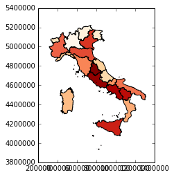
GeoPandas (menzione)
GeoPandas è un'estensione di pandas per agevolare l'utilizzo e visualizzazione di forme geometriche e geografiche nel dataframe:
Se vi interessa:
su SoftPython: c'è una sezione ma è più che altro una bozza
Per tanti bei tutorial completi online: raccomando il materiale (in inglese) dal sito Geospatial Analysis and Representation for Data Science del relativo corso tenuto da Maurizio Napolitano (FBK) al master in Data Science all’Università di Trento.