Analytics with Pandas : 2. Advanced operations
Download exercises zip
Let’s see how to do more advanced operations with pandas, like grouping with groupby, joining tables with merge, and perform geospatial analysis with GeoPandas (only mentioned).
We chose to collect such topics in this notebook as tipically while executing these operations problems are more likely to arise and thus some further internet search is required.
1. Grouping
Reference:
To group items and perform statistics on each group, you can use the groupby method.
Let’s see an example of a possible grouping. First we reload again the astropi.csv described in the previous tutorial
[1]:
import pandas as pd
import numpy as np

df = pd.read_csv('astropi.csv', encoding='UTF-8')
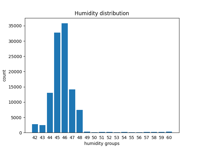
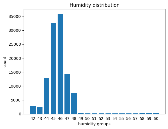
Suppose we want to calculate how many readings of humidity fall into the interval defined by each integer value of humidity humidity_int, so to be able to plot a bar chart like this (actually there are faster methods with numpy for making histograms but here we follow the step by step approach)
1.1 Let’s see a group
To get an initial idea, we could start checking only the rows that belong to the group 42, that is have a humidity value lying between 42.0 included until 43.0 excluded. We can use the transform method as previously seen, noting that group 42 holds 2776 rows:
[2]:
df[ df['humidity'].transform(int) == 42]
[2]:
| time_stamp | temp_cpu | temp_h | temp_p | humidity | pressure | pitch | roll | yaw | mag_x | mag_y | mag_z | accel_x | accel_y | accel_z | gyro_x | gyro_y | gyro_z | reset | |
|---|---|---|---|---|---|---|---|---|---|---|---|---|---|---|---|---|---|---|---|
| 19222 | 2016-02-18 16:37:00 | 33.18 | 28.96 | 26.51 | 42.99 | 1006.10 | 1.19 | 53.23 | 313.69 | 9.081925 | -32.244905 | -35.135448 | -0.000581 | 0.018936 | 0.014607 | 0.000563 | 0.000346 | -0.000113 | 0 |
| 19619 | 2016-02-18 17:43:50 | 33.34 | 29.06 | 26.62 | 42.91 | 1006.30 | 1.50 | 52.54 | 194.49 | -53.197113 | -4.014863 | -20.257249 | -0.000439 | 0.018838 | 0.014526 | -0.000259 | 0.000323 | -0.000181 | 0 |
| 19621 | 2016-02-18 17:44:10 | 33.38 | 29.06 | 26.62 | 42.98 | 1006.28 | 1.01 | 52.89 | 195.39 | -52.911983 | -4.207085 | -20.754475 | -0.000579 | 0.018903 | 0.014580 | 0.000415 | -0.000232 | 0.000400 | 0 |
| 19655 | 2016-02-18 17:49:51 | 33.37 | 29.07 | 26.62 | 42.94 | 1006.28 | 0.93 | 53.21 | 203.76 | -43.124080 | -8.181511 | -29.151436 | -0.000432 | 0.018919 | 0.014608 | 0.000182 | 0.000341 | 0.000015 | 0 |
| 19672 | 2016-02-18 17:52:40 | 33.33 | 29.06 | 26.62 | 42.93 | 1006.24 | 1.34 | 52.71 | 206.97 | -36.893841 | -10.130503 | -31.484077 | -0.000551 | 0.018945 | 0.014794 | -0.000378 | -0.000013 | -0.000101 | 0 |
| ... | ... | ... | ... | ... | ... | ... | ... | ... | ... | ... | ... | ... | ... | ... | ... | ... | ... | ... | ... |
| 110864 | 2016-02-29 09:24:21 | 31.56 | 27.52 | 24.83 | 42.94 | 1005.83 | 1.58 | 49.93 | 129.60 | -15.169673 | -27.642610 | 1.563183 | -0.000682 | 0.017743 | 0.014646 | -0.000264 | 0.000206 | 0.000196 | 0 |
| 110865 | 2016-02-29 09:24:30 | 31.55 | 27.50 | 24.83 | 42.72 | 1005.85 | 1.89 | 49.92 | 130.51 | -15.832622 | -27.729389 | 1.785682 | -0.000736 | 0.017570 | 0.014855 | 0.000143 | 0.000199 | -0.000024 | 0 |
| 110866 | 2016-02-29 09:24:41 | 31.58 | 27.50 | 24.83 | 42.83 | 1005.85 | 2.09 | 50.00 | 132.04 | -16.646212 | -27.719479 | 1.629533 | -0.000647 | 0.017657 | 0.014799 | 0.000537 | 0.000257 | 0.000057 | 0 |
| 110867 | 2016-02-29 09:24:50 | 31.62 | 27.50 | 24.83 | 42.81 | 1005.88 | 2.88 | 49.69 | 133.00 | -17.270447 | -27.793136 | 1.703806 | -0.000835 | 0.017635 | 0.014877 | 0.000534 | 0.000456 | 0.000195 | 0 |
| 110868 | 2016-02-29 09:25:00 | 31.57 | 27.51 | 24.83 | 42.94 | 1005.86 | 2.17 | 49.77 | 134.18 | -17.885872 | -27.824149 | 1.293345 | -0.000787 | 0.017261 | 0.014380 | 0.000459 | 0.000076 | 0.000030 | 0 |
2776 rows × 19 columns
1.2 groupby
We can generlize and associate to each integer group the amount of rows belonging to that group with the groupby method. First let’s make a column holding the integer humidity value for each group:
[3]:
df['humidity_int'] = df['humidity'].transform( lambda x: int(x) )
[4]:
df[ ['time_stamp', 'humidity_int', 'humidity'] ].head()
[4]:
| time_stamp | humidity_int | humidity | |
|---|---|---|---|
| 0 | 2016-02-16 10:44:40 | 44 | 44.94 |
| 1 | 2016-02-16 10:44:50 | 45 | 45.12 |
| 2 | 2016-02-16 10:45:00 | 45 | 45.12 |
| 3 | 2016-02-16 10:45:10 | 45 | 45.32 |
| 4 | 2016-02-16 10:45:20 | 45 | 45.18 |
Then we can call groupby by writing down:
first the column where to group (
humidity_int)second the column where to calculate the statistics
finally the statistics to be performed, in this case
.count()(other common ones aresum(),min(),max(),mean()…)
[5]:
df.groupby(['humidity_int'])['humidity'].count()
[5]:
humidity_int
42     2776
43     2479
44    13029
45    32730
46    35775
47    14176
48     7392
49      297
50      155
51      205
52      209
53      128
54      224
55      164
56      139
57      183
58      237
59      271
60      300
Name: humidity, dtype: int64
Note the result is a Series:
[6]:
result = df.groupby(['humidity_int'])['humidity'].count()
[7]:
type(result)
[7]:
pandas.core.series.Series
Since we would like a customized bar chart, for the sake of simplicity we could use the native plt.plot function of matplotlib, for which we will need one sequence for \(xs\) coordinates and another one for the \(ys\).
The sequence for \(xs\) can be extracted from the index of the Series:
[8]:
result.index
[8]:
Int64Index([42, 43, 44, 45, 46, 47, 48, 49, 50, 51, 52, 53, 54, 55, 56, 57, 58,
            59, 60],
           dtype='int64', name='humidity_int')
For the \(ys\) sequence we can directly use the Series like this:
[9]:
%matplotlib inline
import matplotlib as mpl
import matplotlib.pyplot as plt

plt.bar(result.index, result)

plt.xlabel('humidity groups')
plt.ylabel('count')
plt.title('Humidity distribution')

plt.xticks(result.index, result.index) # shows labels as integers
plt.tick_params(bottom=False)          # removes the little bottom lines


plt.show()
1.3 Modifying a dataframe by plugging in the result of a grouping
Notice we’ve got only 19 rows in the grouped series:
[10]:
df.groupby(['humidity_int'])['humidity'].count()
[10]:
humidity_int
42     2776
43     2479
44    13029
45    32730
46    35775
47    14176
48     7392
49      297
50      155
51      205
52      209
53      128
54      224
55      164
56      139
57      183
58      237
59      271
60      300
Name: humidity, dtype: int64
How could we fill the whole original table, assigning to each row the count of its own group?
We can use transform like this:
[11]:
df.groupby(['humidity_int'])['humidity'].transform('count')
[11]:
0         13029
1         32730
2         32730
3         32730
4         32730
          ...
110864     2776
110865     2776
110866     2776
110867     2776
110868     2776
Name: humidity, Length: 110869, dtype: int64
As usual, group_by does not modify the dataframe, if we want the result stored in the dataframe we need to assign the result to a new column:
[12]:
df['humidity_counts'] = df.groupby(['humidity_int'])['humidity'].transform('count')
[13]:
df
[13]:
| time_stamp | temp_cpu | temp_h | temp_p | humidity | pressure | pitch | roll | yaw | mag_x | ... | mag_z | accel_x | accel_y | accel_z | gyro_x | gyro_y | gyro_z | reset | humidity_int | humidity_counts | |
|---|---|---|---|---|---|---|---|---|---|---|---|---|---|---|---|---|---|---|---|---|---|
| 0 | 2016-02-16 10:44:40 | 31.88 | 27.57 | 25.01 | 44.94 | 1001.68 | 1.49 | 52.25 | 185.21 | -46.422753 | ... | -12.129346 | -0.000468 | 0.019439 | 0.014569 | 0.000942 | 0.000492 | -0.000750 | 20 | 44 | 13029 |
| 1 | 2016-02-16 10:44:50 | 31.79 | 27.53 | 25.01 | 45.12 | 1001.72 | 1.03 | 53.73 | 186.72 | -48.778951 | ... | -12.943096 | -0.000614 | 0.019436 | 0.014577 | 0.000218 | -0.000005 | -0.000235 | 0 | 45 | 32730 |
| 2 | 2016-02-16 10:45:00 | 31.66 | 27.53 | 25.01 | 45.12 | 1001.72 | 1.24 | 53.57 | 186.21 | -49.161878 | ... | -12.642772 | -0.000569 | 0.019359 | 0.014357 | 0.000395 | 0.000600 | -0.000003 | 0 | 45 | 32730 |
| 3 | 2016-02-16 10:45:10 | 31.69 | 27.52 | 25.01 | 45.32 | 1001.69 | 1.57 | 53.63 | 186.03 | -49.341941 | ... | -12.615509 | -0.000575 | 0.019383 | 0.014409 | 0.000308 | 0.000577 | -0.000102 | 0 | 45 | 32730 |
| 4 | 2016-02-16 10:45:20 | 31.66 | 27.54 | 25.01 | 45.18 | 1001.71 | 0.85 | 53.66 | 186.46 | -50.056683 | ... | -12.678341 | -0.000548 | 0.019378 | 0.014380 | 0.000321 | 0.000691 | 0.000272 | 0 | 45 | 32730 |
| ... | ... | ... | ... | ... | ... | ... | ... | ... | ... | ... | ... | ... | ... | ... | ... | ... | ... | ... | ... | ... | ... |
| 110864 | 2016-02-29 09:24:21 | 31.56 | 27.52 | 24.83 | 42.94 | 1005.83 | 1.58 | 49.93 | 129.60 | -15.169673 | ... | 1.563183 | -0.000682 | 0.017743 | 0.014646 | -0.000264 | 0.000206 | 0.000196 | 0 | 42 | 2776 |
| 110865 | 2016-02-29 09:24:30 | 31.55 | 27.50 | 24.83 | 42.72 | 1005.85 | 1.89 | 49.92 | 130.51 | -15.832622 | ... | 1.785682 | -0.000736 | 0.017570 | 0.014855 | 0.000143 | 0.000199 | -0.000024 | 0 | 42 | 2776 |
| 110866 | 2016-02-29 09:24:41 | 31.58 | 27.50 | 24.83 | 42.83 | 1005.85 | 2.09 | 50.00 | 132.04 | -16.646212 | ... | 1.629533 | -0.000647 | 0.017657 | 0.014799 | 0.000537 | 0.000257 | 0.000057 | 0 | 42 | 2776 |
| 110867 | 2016-02-29 09:24:50 | 31.62 | 27.50 | 24.83 | 42.81 | 1005.88 | 2.88 | 49.69 | 133.00 | -17.270447 | ... | 1.703806 | -0.000835 | 0.017635 | 0.014877 | 0.000534 | 0.000456 | 0.000195 | 0 | 42 | 2776 |
| 110868 | 2016-02-29 09:25:00 | 31.57 | 27.51 | 24.83 | 42.94 | 1005.86 | 2.17 | 49.77 | 134.18 | -17.885872 | ... | 1.293345 | -0.000787 | 0.017261 | 0.014380 | 0.000459 | 0.000076 | 0.000030 | 0 | 42 | 2776 |
110869 rows × 21 columns
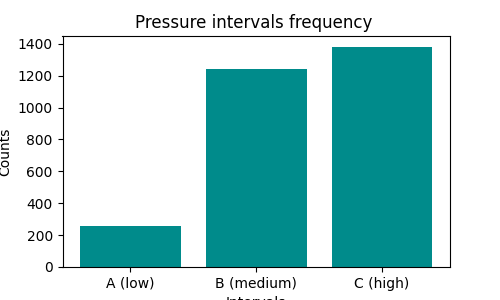
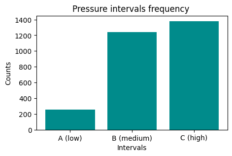
1.4 Exercise - meteo pressure intervals
✪✪✪ The dataset meteo.csv contains the weather data of Trento, November 2017 (source: www.meteotrentino.it). We would like to subdivide the pressure readings into three intervals A (low), B (medium), C (high), and count how many readings have been made for each interval.
IMPORTANT: assign the dataframe to a variable called meteo so to avoid confusion with other dataframes
1.4.1 Where are the intervals?
First, let’s find the pressure values for these 3 intervals and plot them as segments, so to end up with a chart like this:
Before doing the plot, we will need to know at which height we should plot the segments.
Load the dataset with pandas, calculate the following variables and PRINT them
use
UTF-8as encodinground values with
roundfunctionthe excursion is the difference between minimum and maximum
note
intervalCcoincides with the maximum
DO NOT use min and max as variable names (they are reserved functions!!)
[14]:
import pandas as pd
# write here
minimum: 966.3
maximum: 998.3
excursion: 32.0
intervalA: 976.97
intervalB: 987.63
intervalC: 998.3
1.4.2 Segments plot
Try now to plot the chart of pressure and the 4 horizontal segments.
to overlay the segments with different colors, just make repeated calls to
plt.plota segment is defined by two points: so just find the coordinates of those two points..
try leaving some space above and below the chart
REMEMBER title and labels
Show solution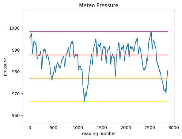
[15]:
# write here

1.4.3 Assigning the intervals
We literally made a picture of where the intervals are located - let’s now ask ourselves how many readings have been done for each interval.
First, try creating a column which assigns to each reading the interval where it belongs to.
HINT 1: use
transformHINT 2: in the function you are going to define, do not recalculate inside values such as minimum, maximum, intervals etc because it would slow down Pandas. Instead, use the variables we’ve already defined - remember that
transformriexecutes the argument function for each row!
[16]:
# write here
[16]:
| Date | Pressure | Rain | Temp | PressureInterval | |
|---|---|---|---|---|---|
| 0 | 01/11/2017 00:00 | 995.4 | 0.0 | 5.4 | C (high) |
| 1 | 01/11/2017 00:15 | 995.5 | 0.0 | 6.0 | C (high) |
| 2 | 01/11/2017 00:30 | 995.5 | 0.0 | 5.9 | C (high) |
| 3 | 01/11/2017 00:45 | 995.7 | 0.0 | 5.4 | C (high) |
| 4 | 01/11/2017 01:00 | 995.7 | 0.0 | 5.3 | C (high) |
| ... | ... | ... | ... | ... | ... |
| 2873 | 30/11/2017 23:00 | 980.0 | 0.0 | 0.2 | B (medium) |
| 2874 | 30/11/2017 23:15 | 980.2 | 0.0 | 0.5 | B (medium) |
| 2875 | 30/11/2017 23:30 | 980.2 | 0.0 | 0.6 | B (medium) |
| 2876 | 30/11/2017 23:45 | 980.5 | 0.0 | 0.2 | B (medium) |
| 2877 | 01/12/2017 00:00 | 980.6 | 0.0 | -0.3 | B (medium) |
2878 rows × 5 columns
1.4.4 Grouping by intervals
We would like to have an histogram like this one:
First, create a grouping to count occurrences:
[17]:
# write here
[17]:
PressureInterval
A (low)        255
B (medium)    1243
C (high)      1380
Name: Pressure, dtype: int64
Now plot it
NOTE: the result of
groupbyis also aSeries, so it’s plottable as we’ve already seen…REMEMBER title and axis labels
[18]:
%matplotlib inline
import matplotlib as mpl
import matplotlib.pyplot as plt

# write here

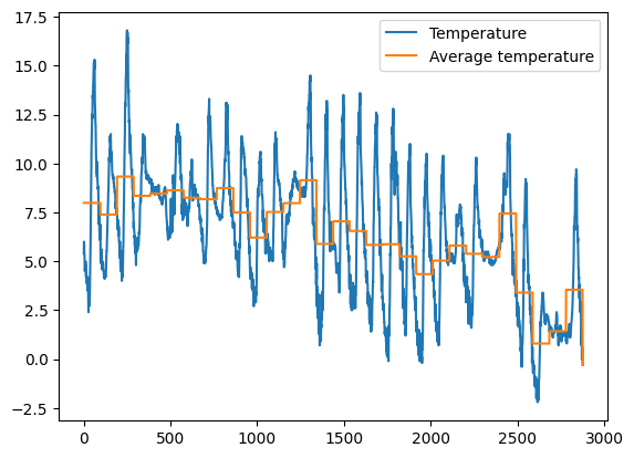
1.5 Exercise - meteo average temperature
✪✪✪ Calculate the average temperature for each day, and show it in the plot, so to have a couple new columns like these:
    Day       Avg_day_temp
01/11/2017      7.983333
01/11/2017      7.983333
01/11/2017      7.983333
    .               .
    .               .
02/11/2017      7.384375
02/11/2017      7.384375
02/11/2017      7.384375
    .               .
    .               .
HINT 1: add 'Day' column by extracting only the day from the date. To do it, use the function .strapplied to all the column.
HINT 2: There are various ways to solve the exercise:
Most perfomant and elegant is with
groupbyoperator, see Pandas trasform - more than meets the eyeAs alternative, you may use a
forto cycle through days. Typically, using aforis not a good idea with Pandas, as on large datasets it can take a lot to perform the updates. Still, since this dataset is small enough, you should get results in a decent amount of time.
[19]:
# write here

[20]:
****SOLUTION 1 (EFFICIENT) -  best solution with groupby and transform
               Date  Pressure  Rain  Temp         Day  Avg_day_temp
0  01/11/2017 00:00     995.4   0.0   5.4  01/11/2017      7.983333
1  01/11/2017 00:15     995.5   0.0   6.0  01/11/2017      7.983333
2  01/11/2017 00:30     995.5   0.0   5.9  01/11/2017      7.983333
3  01/11/2017 00:45     995.7   0.0   5.4  01/11/2017      7.983333
4  01/11/2017 01:00     995.7   0.0   5.3  01/11/2017      7.983333


[21]:
[22]:
2. Merging tables
Suppose we want to add a column with geographical position of the ISS. To do so, we would need to join our dataset with another one containing such information. Let’s take for example the dataset iss-coords.csv
[23]:
iss_coords = pd.read_csv('iss-coords.csv', encoding='UTF-8')
[24]:
iss_coords
[24]:
| timestamp | lat | lon | |
|---|---|---|---|
| 0 | 2016-01-01 05:11:30 | -45.103458 | 14.083858 |
| 1 | 2016-01-01 06:49:59 | -37.597242 | 28.931170 |
| 2 | 2016-01-01 11:52:30 | 17.126141 | 77.535602 |
| 3 | 2016-01-01 11:52:30 | 17.126464 | 77.535861 |
| 4 | 2016-01-01 14:54:08 | 7.259561 | 70.001561 |
| ... | ... | ... | ... |
| 333 | 2016-02-29 13:23:17 | -51.077590 | -31.093987 |
| 334 | 2016-02-29 13:44:13 | 30.688553 | -135.403820 |
| 335 | 2016-02-29 13:44:13 | 30.688295 | -135.403533 |
| 336 | 2016-02-29 18:44:57 | 27.608774 | -130.198781 |
| 337 | 2016-02-29 21:36:47 | 27.325186 | -129.893278 |
338 rows × 3 columns
We notice there is a timestamp column, which unfortunately has a slightly different name that time_stamp column (notice the underscore _) in original astropi dataset:
[25]:
df.info()
<class 'pandas.core.frame.DataFrame'>
RangeIndex: 110869 entries, 0 to 110868
Data columns (total 21 columns):
 #   Column           Non-Null Count   Dtype
---  ------           --------------   -----
 0   time_stamp       110869 non-null  object
 1   temp_cpu         110869 non-null  float64
 2   temp_h           110869 non-null  float64
 3   temp_p           110869 non-null  float64
 4   humidity         110869 non-null  float64
 5   pressure         110869 non-null  float64
 6   pitch            110869 non-null  float64
 7   roll             110869 non-null  float64
 8   yaw              110869 non-null  float64
 9   mag_x            110869 non-null  float64
 10  mag_y            110869 non-null  float64
 11  mag_z            110869 non-null  float64
 12  accel_x          110869 non-null  float64
 13  accel_y          110869 non-null  float64
 14  accel_z          110869 non-null  float64
 15  gyro_x           110869 non-null  float64
 16  gyro_y           110869 non-null  float64
 17  gyro_z           110869 non-null  float64
 18  reset            110869 non-null  int64
 19  humidity_int     110869 non-null  int64
 20  humidity_counts  110869 non-null  int64
dtypes: float64(17), int64(3), object(1)
memory usage: 17.8+ MB
To merge datasets according to the columns, we can use the command merge like this:
[26]:
# remember merge produces a NEW dataframe

geo_astropi = df.merge(iss_coords, left_on='time_stamp', right_on='timestamp')

# merge will add both time_stamp and timestamp columns,
# so we remove the duplicate column `timestamp`
geo_astropi = geo_astropi.drop('timestamp', axis=1)
[27]:
geo_astropi
[27]:
| time_stamp | temp_cpu | temp_h | temp_p | humidity | pressure | pitch | roll | yaw | mag_x | ... | accel_y | accel_z | gyro_x | gyro_y | gyro_z | reset | humidity_int | humidity_counts | lat | lon | |
|---|---|---|---|---|---|---|---|---|---|---|---|---|---|---|---|---|---|---|---|---|---|
| 0 | 2016-02-19 03:49:00 | 32.53 | 28.37 | 25.89 | 45.31 | 1006.04 | 1.31 | 51.63 | 34.91 | 21.125001 | ... | 0.018851 | 0.014607 | 0.000060 | -0.000304 | 0.000046 | 0 | 45 | 32730 | 31.434741 | 52.917464 |
| 1 | 2016-02-19 14:30:40 | 32.30 | 28.12 | 25.62 | 45.57 | 1007.42 | 1.49 | 52.29 | 333.49 | 16.083471 | ... | 0.018687 | 0.014502 | 0.000208 | -0.000499 | 0.000034 | 0 | 45 | 32730 | -46.620658 | -57.311657 |
| 2 | 2016-02-19 14:30:40 | 32.30 | 28.12 | 25.62 | 45.57 | 1007.42 | 1.49 | 52.29 | 333.49 | 16.083471 | ... | 0.018687 | 0.014502 | 0.000208 | -0.000499 | 0.000034 | 0 | 45 | 32730 | -46.620477 | -57.311138 |
| 3 | 2016-02-21 22:14:11 | 32.21 | 28.05 | 25.50 | 47.36 | 1012.41 | 0.67 | 52.40 | 27.57 | 15.441683 | ... | 0.018800 | 0.014136 | -0.000015 | -0.000159 | 0.000221 | 0 | 47 | 14176 | 19.138359 | -140.211489 |
| 4 | 2016-02-23 23:40:50 | 32.32 | 28.18 | 25.61 | 47.45 | 1010.62 | 1.14 | 51.41 | 33.68 | 11.994554 | ... | 0.018276 | 0.014124 | 0.000368 | 0.000368 | 0.000030 | 0 | 47 | 14176 | 4.713819 | 80.261665 |
| 5 | 2016-02-24 10:05:51 | 32.39 | 28.26 | 25.70 | 46.83 | 1010.51 | 0.61 | 51.91 | 287.86 | 6.554283 | ... | 0.018352 | 0.014344 | -0.000664 | -0.000518 | 0.000171 | 0 | 46 | 35775 | -46.061583 | 22.246025 |
| 6 | 2016-02-25 00:23:01 | 32.38 | 28.18 | 25.62 | 46.52 | 1008.28 | 0.90 | 51.77 | 30.80 | 9.947132 | ... | 0.018502 | 0.014366 | 0.000290 | 0.000314 | -0.000375 | 0 | 46 | 35775 | 47.047346 | 137.958918 |
| 7 | 2016-02-27 01:43:10 | 32.42 | 28.34 | 25.76 | 45.72 | 1006.79 | 0.57 | 49.85 | 10.57 | 7.805606 | ... | 0.017930 | 0.014378 | -0.000026 | -0.000013 | -0.000047 | 0 | 45 | 32730 | -41.049112 | 30.193004 |
| 8 | 2016-02-27 01:43:10 | 32.42 | 28.34 | 25.76 | 45.72 | 1006.79 | 0.57 | 49.85 | 10.57 | 7.805606 | ... | 0.017930 | 0.014378 | -0.000026 | -0.000013 | -0.000047 | 0 | 45 | 32730 | -8.402991 | -100.981726 |
| 9 | 2016-02-28 09:48:40 | 32.62 | 28.62 | 26.02 | 45.15 | 1006.06 | 1.12 | 50.44 | 301.74 | 10.348327 | ... | 0.017620 | 0.014725 | -0.000358 | -0.000301 | -0.000061 | 0 | 45 | 32730 | 50.047523 | 175.566751 |
10 rows × 23 columns
Exercise 2.1 - better merge
If you notice, above table does have lat and lon columns, but has very few rows. Why ? Try to merge the tables in some meaningful way so to have all the original rows and all cells of lat and lon filled.
For other merging stategies, read about attribute
howin Why And How To Use Merge With Pandas in PythonTo fill missing values don’t use fancy interpolation techniques, just put the station position in that given day or hour
[28]:
# write here
[28]:
| time_stamp | temp_cpu | temp_h | temp_p | humidity | pressure | pitch | roll | yaw | mag_x | ... | accel_z | gyro_x | gyro_y | gyro_z | reset | humidity_int | humidity_counts | timestamp | lat | lon | |
|---|---|---|---|---|---|---|---|---|---|---|---|---|---|---|---|---|---|---|---|---|---|
| 0 | 2016-02-16 10:44:40 | 31.88 | 27.57 | 25.01 | 44.94 | 1001.68 | 1.49 | 52.25 | 185.21 | -46.422753 | ... | 0.014569 | 0.000942 | 0.000492 | -0.000750 | 20 | 44 | 13029 | NaN | NaN | NaN |
| 1 | 2016-02-16 10:44:50 | 31.79 | 27.53 | 25.01 | 45.12 | 1001.72 | 1.03 | 53.73 | 186.72 | -48.778951 | ... | 0.014577 | 0.000218 | -0.000005 | -0.000235 | 0 | 45 | 32730 | NaN | NaN | NaN |
| 2 | 2016-02-16 10:45:00 | 31.66 | 27.53 | 25.01 | 45.12 | 1001.72 | 1.24 | 53.57 | 186.21 | -49.161878 | ... | 0.014357 | 0.000395 | 0.000600 | -0.000003 | 0 | 45 | 32730 | NaN | NaN | NaN |
| 3 | 2016-02-16 10:45:10 | 31.69 | 27.52 | 25.01 | 45.32 | 1001.69 | 1.57 | 53.63 | 186.03 | -49.341941 | ... | 0.014409 | 0.000308 | 0.000577 | -0.000102 | 0 | 45 | 32730 | NaN | NaN | NaN |
| 4 | 2016-02-16 10:45:20 | 31.66 | 27.54 | 25.01 | 45.18 | 1001.71 | 0.85 | 53.66 | 186.46 | -50.056683 | ... | 0.014380 | 0.000321 | 0.000691 | 0.000272 | 0 | 45 | 32730 | NaN | NaN | NaN |
| ... | ... | ... | ... | ... | ... | ... | ... | ... | ... | ... | ... | ... | ... | ... | ... | ... | ... | ... | ... | ... | ... |
| 110866 | 2016-02-29 09:24:21 | 31.56 | 27.52 | 24.83 | 42.94 | 1005.83 | 1.58 | 49.93 | 129.60 | -15.169673 | ... | 0.014646 | -0.000264 | 0.000206 | 0.000196 | 0 | 42 | 2776 | NaN | NaN | NaN |
| 110867 | 2016-02-29 09:24:30 | 31.55 | 27.50 | 24.83 | 42.72 | 1005.85 | 1.89 | 49.92 | 130.51 | -15.832622 | ... | 0.014855 | 0.000143 | 0.000199 | -0.000024 | 0 | 42 | 2776 | NaN | NaN | NaN |
| 110868 | 2016-02-29 09:24:41 | 31.58 | 27.50 | 24.83 | 42.83 | 1005.85 | 2.09 | 50.00 | 132.04 | -16.646212 | ... | 0.014799 | 0.000537 | 0.000257 | 0.000057 | 0 | 42 | 2776 | NaN | NaN | NaN |
| 110869 | 2016-02-29 09:24:50 | 31.62 | 27.50 | 24.83 | 42.81 | 1005.88 | 2.88 | 49.69 | 133.00 | -17.270447 | ... | 0.014877 | 0.000534 | 0.000456 | 0.000195 | 0 | 42 | 2776 | NaN | NaN | NaN |
| 110870 | 2016-02-29 09:25:00 | 31.57 | 27.51 | 24.83 | 42.94 | 1005.86 | 2.17 | 49.77 | 134.18 | -17.885872 | ... | 0.014380 | 0.000459 | 0.000076 | 0.000030 | 0 | 42 | 2776 | NaN | NaN | NaN |
110871 rows × 24 columns
3. GeoPandas
You can easily manipulate geographical data with GeoPandas library. For some nice online tutorial, we refer to Geospatial Analysis and Representation for Data Science course website @ master in Data Science University of Trento, by Maurizio Napolitano (FBK)
Continue
Go on with the challenges worksheet