Relational data 3 - simple statistics

Download exercises zip

Browse files online

We will now compute and visualize simple statistics about graphs (they don’t require node discovery algorithms).

What to do

• unzip exercises in a folder, you should get something like this:

relational
    relational1-intro.ipynb
    relational1-intro-sol.ipynb
    relational2-binrel.ipynb
    relational2-binrel-sol.ipynb
    relational3-simple-stats.ipynb
    relational3-simple-stats-sol.ipynb
    relational4-chal.ipynb
    jupman.py
    soft.py

WARNING: to correctly visualize the notebook, it MUST be in an unzipped folder !

• open Jupyter Notebook from that folder. Two things should open, first a console and then browser. The browser should show a file list: navigate the list and open the notebook relational/relational3-simple-stats.ipynb

WARNING 2: DO NOT use the Upload button in Jupyter, instead navigate in Jupyter browser to the unzipped folder !

• Go on reading that notebook, and follow instuctions inside.

Shortcut keys:

• to execute Python code inside a Jupyter cell, press Control + Enter

• to execute Python code inside a Jupyter cell AND select next cell, press Shift + Enter

• to execute Python code inside a Jupyter cell AND a create a new cell aftwerwards, press Alt + Enter

• If the notebooks look stuck, try to select Kernel -> Restart

Outdegrees and indegrees

The out-degree \(\deg^+(v)\) of a node \(v\) is the number of edges going out from it, while the in-degree \(\deg^-(v)\) is the number of edges going into it.

NOTE: the out-degree and in-degree are not the sum of weights ! They just count presence or absence of edges.

For example, consider this graph:

from soft import draw_adj

d = {
    'a' : ['b','c'],
    'b' : ['b','d'],
    'c' : ['a','b','c','d'],
    'd' : ['b','d']
}


draw_adj(d)

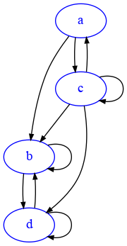
The out-degree of d is 2, because it has one outgoing edge to b but also an outgoing edge to itself. The indegree of d is 3, because it has an edge coming from b, one from c and one self-loop from d itself.

Exercise - outdegree_adj

✪ RETURN the outdegree of a node from graph d represented as a dictionary of adjacency lists

• If v is not a vertex of d, raise ValueError

Show solution

def outdegree_adj(d, v):

    if v not in d:
        raise ValueError("Vertex %s is not in %s" % (v, d))

    return len(d[v])


try:
    outdegree_adj({'a':[]},'b')
    raise Exception("SHOULD HAVE FAILED !")
except ValueError:
    "passed test"

d1 = { 'a':[] }
assert outdegree_adj(d1,'a') == 0

d2 = { 'a':['a'] }
assert outdegree_adj(d2,'a') == 1

d3 = { 'a':['a','b'],
       'b':[] }
assert outdegree_adj(d3,'a') == 2

d4 = { 'a':['a','b'],
       'b':['a','b','c'],
       'c':[] }
assert outdegree_adj(d4,'b') == 3

def outdegree_adj(d, v):
    raise Exception('TODO IMPLEMENT ME !')

try:
    outdegree_adj({'a':[]},'b')
    raise Exception("SHOULD HAVE FAILED !")
except ValueError:
    "passed test"

d1 = { 'a':[] }
assert outdegree_adj(d1,'a') == 0

d2 = { 'a':['a'] }
assert outdegree_adj(d2,'a') == 1

d3 = { 'a':['a','b'],
       'b':[] }
assert outdegree_adj(d3,'a') == 2

d4 = { 'a':['a','b'],
       'b':['a','b','c'],
       'c':[] }
assert outdegree_adj(d4,'b') == 3

Exercise - outdegree_mat

✪✪ RETURN the outdegree of a node i from a graph boolean matrix \(n\) x \(n\) represented as a list of lists

• If i is not a node of the graph, raise ValueError

Show solution

def outdegree_mat(mat, i):

    n = len(mat)
    if i < 0 or i > n:
        raise ValueError("i %s is not a row of matrix %s" % (i, mat))
    ret = 0
    for j in range(n):
        if mat[i][j]:
            ret += 1
    return ret


try:
    outdegree_mat([[False]],7)
    raise Exception("SHOULD HAVE FAILED !")
except ValueError:
    "passed test"

try:
    outdegree_mat([[False]],-1)
    raise Exception("SHOULD HAVE FAILED !")
except ValueError:
    "passed test"

m1 = [ [False] ]
assert outdegree_mat( m1, 0) == 0

m2 = [ [True] ]
assert outdegree_mat( m2, 0) == 1

m3 = [ [True, True],
       [False, False] ]
assert outdegree_mat( m3, 0) == 2

m4 = [ [True, True, False],
       [True, True, True],
       [False, False, False] ]
assert outdegree_mat(m4,1) == 3

def outdegree_mat(mat, i):
    raise Exception('TODO IMPLEMENT ME !')

try:
    outdegree_mat([[False]],7)
    raise Exception("SHOULD HAVE FAILED !")
except ValueError:
    "passed test"

try:
    outdegree_mat([[False]],-1)
    raise Exception("SHOULD HAVE FAILED !")
except ValueError:
    "passed test"

m1 = [ [False] ]
assert outdegree_mat( m1, 0) == 0

m2 = [ [True] ]
assert outdegree_mat( m2, 0) == 1

m3 = [ [True, True],
       [False, False] ]
assert outdegree_mat( m3, 0) == 2

m4 = [ [True, True, False],
       [True, True, True],
       [False, False, False] ]
assert outdegree_mat(m4,1) == 3

Exercise - outdegree_avg

✪✪ RETURN the average outdegree of nodes in graph d, represented as dictionary of adjacency lists.

• Assume all nodes are in the keys.

Show solution

def outdegree_avg(d):

    s = 0
    for k in d:
        s += len(d[k])
    return s / len(d)


d1 = { 'a':[] }
assert outdegree_avg(d1) == 0

d2 = { 'a':['a'] }
assert round( outdegree_avg(d2), 2) == 1.00 / 1.00

d3 = { 'a':['a','b'],
       'b':[] }
assert round( outdegree_avg(d3), 2) == (2 + 0) / 2

d4 = { 'a':['a','b'],
       'b':['a','b','c'],
       'c':[] }
assert round( outdegree_avg(d4), 2) == round( (2 + 3) / 3 , 2)

def outdegree_avg(d):
    raise Exception('TODO IMPLEMENT ME !')

d1 = { 'a':[] }
assert outdegree_avg(d1) == 0

d2 = { 'a':['a'] }
assert round( outdegree_avg(d2), 2) == 1.00 / 1.00

d3 = { 'a':['a','b'],
       'b':[] }
assert round( outdegree_avg(d3), 2) == (2 + 0) / 2

d4 = { 'a':['a','b'],
       'b':['a','b','c'],
       'c':[] }
assert round( outdegree_avg(d4), 2) == round( (2 + 3) / 3 , 2)

Exercise - indegree_adj

The indegree of a node v is the number of edges going into it.

✪✪ RETURN the indegree of node v in graph d, represented as a dictionary of adjacency lists

• If v is not a node of the graph, raise ValueError

Show solution

def indegree_adj(d, v):

    if v not in d:
        raise ValueError("Vertex %s is not in %s" % (v, d))
    ret = 0
    for k in d:
        if v in d[k]:
            ret += 1
    return ret


try:
    indegree_adj({'a':[]},'b')
    raise Exception("SHOULD HAVE FAILED !")
except ValueError:
    "passed test"

d1 = { 'a':[] }
assert indegree_adj(d1,'a') == 0

d2 = {'a':['a']}
assert indegree_adj(d2,'a') == 1

d3 = { 'a':['a','b'],
       'b':[]}
assert indegree_adj(d3, 'a') == 1

d4 = { 'a':['a','b'],
       'b':['a','b','c'],
       'c':[]}
assert indegree_adj(d4, 'b') == 2

def indegree_adj(d, v):
    raise Exception('TODO IMPLEMENT ME !')

try:
    indegree_adj({'a':[]},'b')
    raise Exception("SHOULD HAVE FAILED !")
except ValueError:
    "passed test"

d1 = { 'a':[] }
assert indegree_adj(d1,'a') == 0

d2 = {'a':['a']}
assert indegree_adj(d2,'a') == 1

d3 = { 'a':['a','b'],
       'b':[]}
assert indegree_adj(d3, 'a') == 1

d4 = { 'a':['a','b'],
       'b':['a','b','c'],
       'c':[]}
assert indegree_adj(d4, 'b') == 2

Exercise - indegree_mat

✪✪ RETURN the indegree of a node i from a graph boolean matrix nxn represented as a list of lists

• If i is not a node of the graph, raise ValueError

Show solution

def indegree_mat(mat, i):

    n = len(mat)
    if i < 0 or i > n:
        raise ValueError("i %s is not a row of matrix %s" % (i, mat))
    ret = 0
    for k in range(n):
        if mat[k][i]:
            ret += 1
    return ret


try:
    indegree_mat([[False]],7)
    raise Exception("SHOULD HAVE FAILED !")
except ValueError:
    "passed test"

assert indegree_mat(
        [
            [False]
        ]
,0) == 0

m1 = [ [True] ]
assert indegree_mat(m1, 0) == 1

m2 = [ [True, True],
       [False, False] ]
assert indegree_mat(m2, 0) == 1

m3 = [ [True, True, False],
       [True, True, True],
       [False, False, False] ]
assert indegree_mat( m3, 1) == 2

def indegree_mat(mat, i):
    raise Exception('TODO IMPLEMENT ME !')

try:
    indegree_mat([[False]],7)
    raise Exception("SHOULD HAVE FAILED !")
except ValueError:
    "passed test"

assert indegree_mat(
        [
            [False]
        ]
,0) == 0

m1 = [ [True] ]
assert indegree_mat(m1, 0) == 1

m2 = [ [True, True],
       [False, False] ]
assert indegree_mat(m2, 0) == 1

m3 = [ [True, True, False],
       [True, True, True],
       [False, False, False] ]
assert indegree_mat( m3, 1) == 2

Exercise - indegree_avg

✪✪ RETURN the average indegree of nodes in graph d, represented as dictionary of adjacency lists.

• Assume all nodes are in the keys

Show solution

def indegree_avg(d):

    s = 0
    for k in d:
        s += len(d[k])
    return s / len(d)


d1 = { 'a':[] }
assert indegree_avg(d1) == 0

d2 = { 'a':['a'] }
assert round( indegree_avg(d2), 2) == 1.00 / 1.00

d3 = { 'a':['a','b'],
       'b':[]}
assert round( indegree_avg(d3), 2) == (1 + 1) / 2

d4 = { 'a':['a','b'],
       'b':['a','b','c'],
       'c':[]}
assert round( indegree_avg(d4), 2) == round( (2 + 2 + 1) / 3 , 2)

def indegree_avg(d):
    raise Exception('TODO IMPLEMENT ME !')

d1 = { 'a':[] }
assert indegree_avg(d1) == 0

d2 = { 'a':['a'] }
assert round( indegree_avg(d2), 2) == 1.00 / 1.00

d3 = { 'a':['a','b'],
       'b':[]}
assert round( indegree_avg(d3), 2) == (1 + 1) / 2

d4 = { 'a':['a','b'],
       'b':['a','b','c'],
       'c':[]}
assert round( indegree_avg(d4), 2) == round( (2 + 2 + 1) / 3 , 2)

Was it worth it?

QUESTION: Is there any difference between the results of indegree_avg and outdegree_avg ?

Show answer

ANSWER: They give the same result. Think about what you did: for outdegree_avg you summed over all rows and then divided by n. For indegree_avg you summed over all columns, and then divided by n.

More formally, we have that the so-called degree sum formula holds (see Wikipedia for more info):

\(\sum_{v \in V} \deg^-(v) = \sum_{v \in V} \deg^+(v) = |A|\)

networkx Indegrees and outdegrees

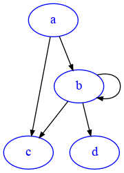
With Networkx we can easily calculate indegrees and outdegrees of a node:

import networkx as nx

# notice with networkx if nodes are already referenced to in an adjacency list
# you do not need to put them as keys:

G=nx.DiGraph({
    'a':['b','c'],        # node a links to b and c
    'b':['b','c', 'd']    # node b links to b itself, c and d
})

draw_nx(G)

G.out_degree('a')

2

QUESTION: What is the outdegree of 'b' ? Try to think about it and then confirm your thoughts with networkx:

Show solution

# write here
#print("indegree  b:  %s" % G.in_degree('b'))
#print("outdegree b:  %s" % G.out_degree('b'))

# write here

QUESTION: We defined indegree and outdegree. Can you guess what the degree might be ? In particular, for a self pointing node like 'b', what could it be? Try to use G.degree('b') methods to validate your thoughts.

Show solution

# write here
#print("degree  b:  %s" % G.degree('b'))

# write here

Show answer

ANSWER: it is the sum of indegree and outdegree. In presence of a self-loop like for 'b', we count the self-loop twice, once as outgoing edge and one as incident edge

Show solution

# write here
#G.degree('b')

# write here

Visualizing distributions

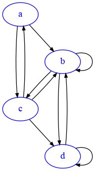
We will try to study the distributions visually. Let’s take an example networkx DiGraph:

import networkx as nx

G1=nx.DiGraph({
    'a':['b','c'],
    'b':['b','c', 'd'],
    'c':['a','b','d'],
    'd':['b', 'd']
})

draw_nx(G1)

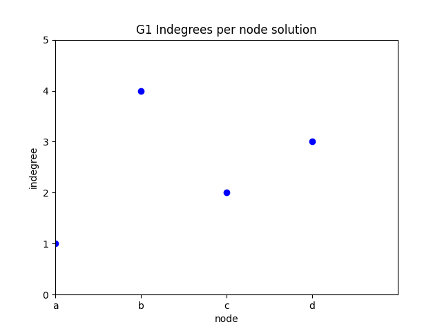
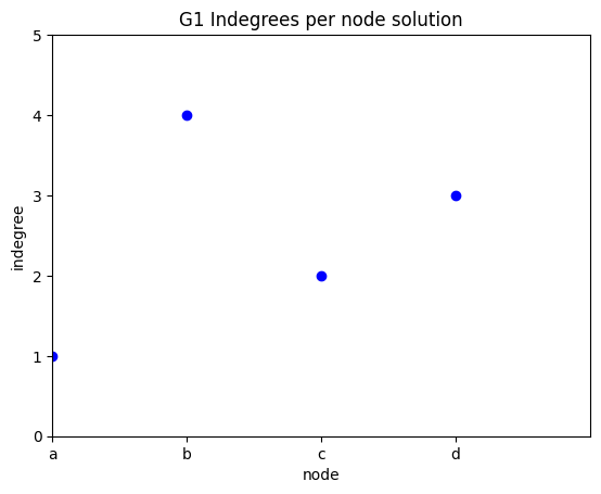
indegree per node

✪✪ Display a plot for graph G where the xtick labels are the nodes, and the y is the indegree of those nodes.

Note: instead of xticks you might directly use categorical variables IF you have matplotlib >= 2.1.0

Here we use xticks as sometimes you might need to fiddle with them anyway

Expected result:

To get the nodes, you can use the G1.nodes() function:

G1.nodes()

NodeView(('a', 'b', 'c', 'd'))

It gives back a NodeView which is not a list, but still you can iterate through it with a for in cycle:

for n in G1.nodes():
    print(n)

a
b
c
d

Also, you can get the indegree of a node with

G1.in_degree('b')

4

Show solution

# write here

import numpy as np
import matplotlib.pyplot as plt

xs = np.arange(G1.number_of_nodes())
ys_in = [G1.in_degree(n) for n in G1.nodes() ]

plt.plot(xs, ys_in,  'bo')

plt.ylim(0,max(ys_in) + 1)
plt.xlim(0,max(xs) + 1)

plt.title("G1 Indegrees per node solution")

plt.xticks(xs, G1.nodes())

plt.xlabel('node')
plt.ylabel('indegree')



plt.show()

# write here

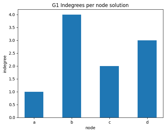
indegree per node bar plot

The previous plot with dots doesn’t look so good - we might try to use instead a bar plot. First look at this example, then proceed with the exercise

✪✪ Display a bar plot for graph G1 where the xtick labels are the nodes, and the y is the indegree of those nodes.

Expected result:

Show solution

# write here

import numpy as np
import matplotlib.pyplot as plt

xs = np.arange(G1.number_of_nodes())
ys_in = [G1.in_degree(n) for n in G1.nodes() ]

plt.bar(xs, ys_in, 0.5, align='center')

plt.title("G1 Indegrees per node solution")
plt.xticks(xs, G1.nodes())

plt.xlabel('node')
plt.ylabel('indegree')


plt.show()

# write here

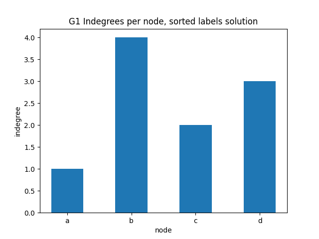
indegree per node sorted alphabetically

✪✪ Display the same bar plot as before, but now sort nodes alphabetically.

NOTE: you cannot run .sort() method on the result given by G1.nodes(), because nodes in network by default have no inherent order. To use .sort() you need first to convert the result to a list object.

You should get something like this:

Show solution

# write here

import numpy as np
import matplotlib.pyplot as plt

xs = np.arange(G1.number_of_nodes())

xs_labels = list(G1.nodes())

xs_labels.sort()

ys_in = [G1.in_degree(n) for n in xs_labels ]

plt.bar(xs, ys_in, 0.5, align='center')

plt.title("G1 Indegrees per node, sorted labels solution")
plt.xticks(xs, xs_labels)

plt.xlabel('node')
plt.ylabel('indegree')


plt.show()

# write here

# write here

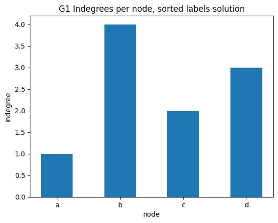
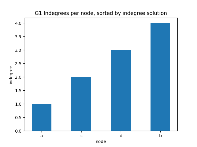
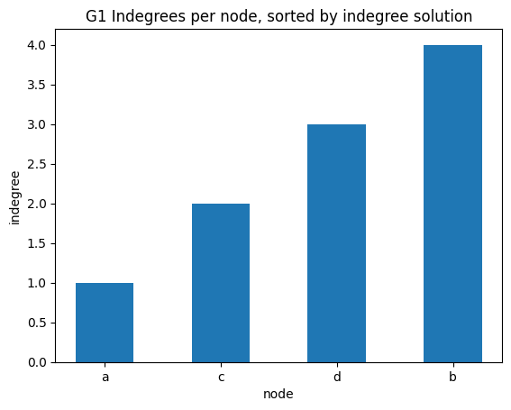
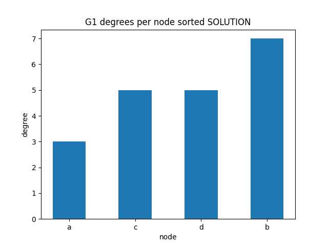
indegree per node sorted

✪✪✪ Display the same bar plot as before, but now sort nodes according to their indegree. This is more challenging, to do it you need to use some sort trick.

• HINT: first read the Python documentation

Expected result:

Show solution

# write here

import numpy as np
import matplotlib.pyplot as plt

xs = np.arange(G1.number_of_nodes())

coords = [(v, G1.in_degree(v)) for v in G1.nodes() ]

coords.sort(key=lambda c: c[1])

ys_in = [c[1] for c in coords]

plt.bar(xs, ys_in, 0.5, align='center')

plt.title("G1 Indegrees per node, sorted by indegree solution")
plt.xticks(xs, [c[0] for c in coords])

plt.xlabel('node')
plt.ylabel('indegree')


plt.show()

# write here

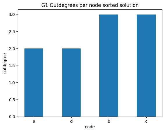
out degrees per node sorted

✪✪✪ Do the same graph as before for the outdegrees.

Expected result:

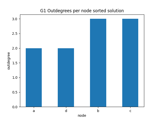
You can get the outdegree of a node with:

G1.out_degree('b')

3

Show solution

# write here
import numpy as np
import matplotlib.pyplot as plt

xs = np.arange(G1.number_of_nodes())

coords = [(v, G1.out_degree(v)) for v in G1.nodes() ]

coords.sort(key=lambda c: c[1])

ys_out = [c[1] for c in coords]

plt.bar(xs, ys_out, 0.5, align='center')

plt.title("G1 Outdegrees per node sorted solution")
plt.xticks(xs, [c[0] for c in coords])

plt.xlabel('node')
plt.ylabel('outdegree')



plt.show()

# write here

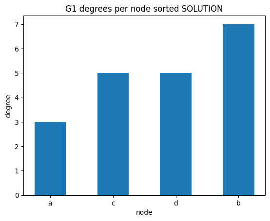
degrees per node

✪✪✪ We might check as well the sorted degrees per node, intended as the sum of in_degree and out_degree. To get the sum, use G1.degree(node) function.

Expected result:

Show solution

# write here

import numpy as np
import matplotlib.pyplot as plt

xs = np.arange(G1.number_of_nodes())

coords = [(v, G1.degree(v)) for v in G1.nodes() ]

coords.sort(key=lambda c: c[1])

ys_deg = [c[1] for c in coords]

plt.bar(xs, ys_deg, 0.5, align='center')

plt.title("G1 degrees per node sorted SOLUTION")
plt.xticks(xs, [c[0] for c in coords])

plt.xlabel('node')
plt.ylabel('degree')


plt.show()

# write here

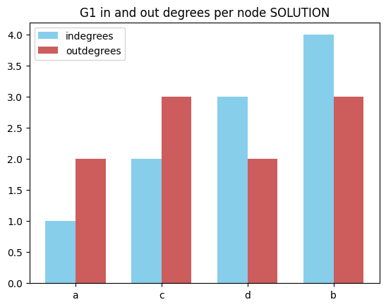
In out degrees per node

✪✪✪✪ Look at this example, and make a double bar chart sorting nodes by their total degree. To do so, in the tuples you will need vertex, in_degree, out_degree and also degree.

Show solution

# write here

import numpy as np
import matplotlib.pyplot as plt

xs = np.arange(G1.number_of_nodes())

coords = [(v, G1.degree(v), G1.in_degree(v), G1.out_degree(v) ) for v in G1.nodes() ]

coords.sort(key=lambda c: c[1])

ys_deg = [c[1] for c in coords]
ys_in = [c[2] for c in coords]
ys_out = [c[3] for c in coords]


width = 0.35
fig, ax = plt.subplots()
rects1 = ax.bar(xs - width/2, ys_in, width,
                color='SkyBlue', label='indegrees')
rects2 = ax.bar(xs + width/2, ys_out, width,
                color='IndianRed', label='outdegrees')

# Add some text for labels, title and custom x-axis tick labels, etc.
ax.set_title('G1 in and out degrees per node SOLUTION')
ax.set_xticks(xs)
ax.set_xticklabels([c[0] for c in coords])
ax.legend()



plt.show()

# write here

Frequency histogram

Now let’s try drawing degree frequencies: for each degree present in the graph we want to display a bar as high as the number of times that particular degree appears.

For doing so, we will need a matplot histogram, see documentation

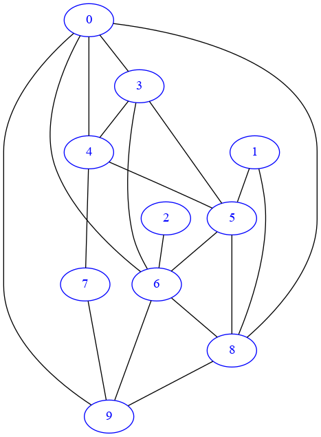
We will need to tell matplotlib how many columns we want, which in histogram terms are called bins. We also need to give the histogram a series of numbers so it can count how many times each number occurs. Let’s consider this graph G2:

import networkx as nx

G2=nx.DiGraph({
    'a':['b','c'],
    'b':['b','c', 'd'],
    'c':['a','b','d'],
    'd':['b', 'd','e'],
    'e':[],
    'f':['c','d','e'],
    'g':['e','g']
})


draw_nx(G2)

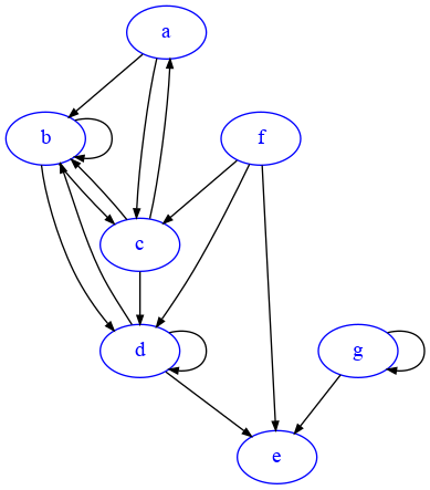
If we take the degree sequence of G2 we get this:

degrees_G2 = [G2.degree(n) for n in G2.nodes()]

degrees_G2

[3, 7, 6, 7, 3, 3, 3]

We see 3 appears four times, 6 once, and 7 twice.

Let’s find a good number for the bins. First we can check the boundaries our x axis should have:

min(degrees_G2)

3

max(degrees_G2)

7

So on the x axis our histogram must go at least from 3 and at least to 7. If we want integer columns (bins), we will need at least ticks for going from 3 included to 7 included, that is at least ticks for 3,4,5,6,7. For precise display, when we have integer x it’s best to also manually provide the sequence of bin edges, remembering it should start at least from the minimum included (in our case, 3) and arrive to the maximum + 1 included (in our case, 7 + 1 = 8)

NOTE: precise histogram drawing can be quite tricky, please do read this StackOverflow post for more details about it.

import matplotlib.pyplot as plt
import numpy as np

degrees = [G2.degree(n) for n in G2.nodes()]

# add histogram

# in this case hist returns a tuple of three values
# we put in three variables
n, bins, columns = plt.hist(degrees_G2,
                            bins=range(3,9), # 3 *included*, 4,5,6,7,8 *included*
                            width=1.0)       # graphical bars width

plt.xlabel('Degrees')
plt.ylabel('Frequency counts')
plt.title('G2 Degree distribution')
plt.xlim(0, max(degrees) + 2)
plt.show()

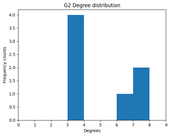
As expected, we see 3 is counted four times, 6 once, and 7 twice.

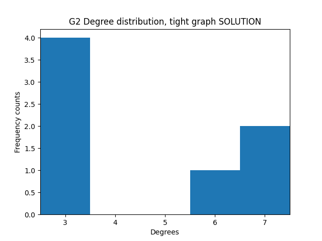
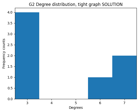
Exercise - better histogram display

✪✪✪ Still, it would be visually better to align the x ticks to the middle of the bars with xticks, and also to make the graph tighter by setting the xlim appropriately. This is not always easy to do.

Read carefully this StackOverflow post and try doing it by yourself.

NOTE: set one thing at a time and try if it works(i.e. first xticks and then xlim), doing everything at once might get quite confusing.

Expected result:

Show solution

# write here

import matplotlib.pyplot as plt
import numpy as np

degrees = [G2.degree(n) for n in G2.nodes()]

# add histogram

min_x = min(degrees)      # 3
max_x = max(degrees)      # 7
bar_width = 1.0

# in this case hist returns a tuple of three values
# we put in three variables
n, bins, columns = plt.hist(
    degrees_G2,
    bins= range(3,9), # 3 *included* to  9 *excluded*
                      # it's like the xs, but with one number more !!
                      # to understand why read this
                      # https://stackoverflow.com/questions/27083051/matplotlib-xticks-not-lining-up-with-histogram/27084005#27084005
    width=bar_width)  #  graphical width of the bars

plt.xlabel('Degrees')
plt.ylabel('Frequency counts')
plt.title('G2 Degree distribution, tight graph SOLUTION')


xs = np.arange(min_x,max_x + 1)  # 3 *included* to 8 *excluded*
                                 # used numpy so we can later reuse it for float vector operations

plt.xticks(xs + bar_width / 2,  # position of ticks
           xs )                 # labels of ticks
plt.xlim(min_x, max_x + 1)  #  3 *included* to 8 *excluded*



plt.show()

# write here

Graph models

Let’s study frequencies of some known network types.

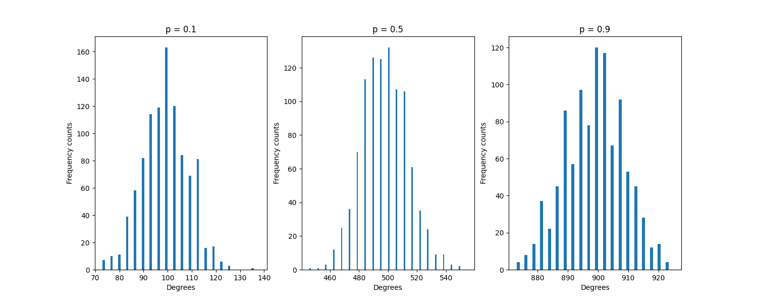
Exercise - Erdős–Rényi model

✪✪ A simple graph model we can think of is the so-called Erdős–Rényi model: it’s an undirected graph where have n nodes, and each node is connected to each other with probability p. In networkx, we can generate a random one by issuing this command:

G = nx.erdos_renyi_graph(10, 0.5)

In the drawing, the absence of arrows confirms it’s undirected:

draw_nx(G)

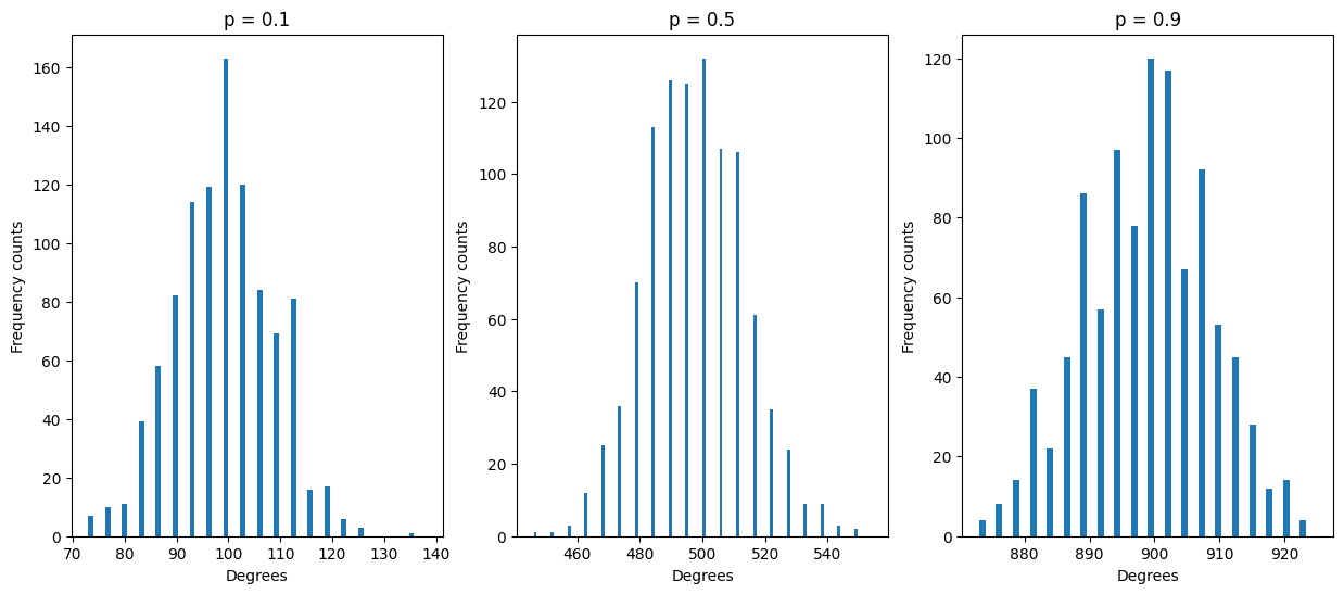
Try plotting degree distribution for different values of p (0.1, 0.5, 0.9) with a fixed n=1000, putting them side by side on the same row. What does their distribution look like ? Where are they centered ?

• to put them side by side, look at this example

• to avoid rewriting the same code again and again, define a plot_erdos(n,p,j) function to be called three times.

Expected result:

Show solution

# write here

import matplotlib.pyplot as plt
import numpy as np

def plot_erdos(n, p, j):
    G = nx.erdos_renyi_graph(n, p)

    plt.subplot(1,   # 1 row
                3,   # 3 columns
                j)   # plotting in jth cell

    degrees = [G.degree(n) for n in G.nodes()]
    num_bins = 20

    n, bins, columns = plt.hist(degrees, num_bins,  width=1.0)

    plt.xlabel('Degrees')
    plt.ylabel('Frequency counts')
    plt.title('p = %s' % p)

n = 1000

fig = plt.figure(figsize=(15,6))  # width: 10 inches, height 3 inches

plot_erdos(n, 0.1, 1)
plot_erdos(n, 0.5, 2)
plot_erdos(n, 0.9, 3)

print()
print("                            Erdős–Rényi degree distribution SOLUTION")



plt.show()

                            Erdős–Rényi degree distribution SOLUTION

# write here

Continue

Go on with the challenges